Golan Levin and Collaborators

• Peer-Reviewed Publications
• Essays and Statements
• Interviews and Dialogues
• Catalogues and Lists
• Project Reports
• Press Clippings
• Lectures
• Code
• Misc.

• 07 2006. Shaping Functions: Polynomial
  
• 07 2006. Shaping Functions: Exponential
  
• 07 2006. Shaping Functions: Circular and Elliptical
  
• 07 2006. Shaping Functions: Bezier and Parametric
  

Exponential Shaping Functions

• Exponential Ease-In and Ease-Out
• Double-Exponential Seat
• Double-Exponential Sigmoid
• The Logistic Sigmoid

Exponential Ease-In and Ease-Out

In this implementation of an exponential shaping function, the control parameter a permits the designer to vary the function from an ease-out form to an ease-in form.

Exponential Ease-In:

Exponential Ease-Out:

//-----------------------------------------
float exponentialEasing (float x, float a){
  
  float epsilon = 0.00001;
  float min_param_a = 0.0 + epsilon;
  float max_param_a = 1.0 - epsilon;
  a = max(min_param_a, min(max_param_a, a));
  
  if (a < 0.5){
    // emphasis
    a = 2.0*(a);
    float y = pow(x, a);
    return y;
  } else {
    // de-emphasis
    a = 2.0*(a-0.5);
    float y = pow(x, 1.0/(1-a));
    return y;
  }
}

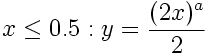
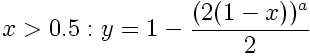
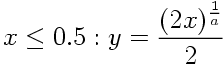
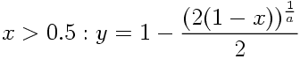
Double-Exponential Seat

A seat-shaped function can be created with a coupling of two exponential functions. This has nicer derivatives than the cubic function, and more continuous control in some respects, at the expense of greater CPU cycles. The recommended range for the control parameter a is from 0 to 1. Note that these equations are very similar to the Double-Exponential Sigmoid described below.

//---------------------------------------------
float doubleExponentialSeat (float x, float a){

  float epsilon = 0.00001;
  float min_param_a = 0.0 + epsilon;
  float max_param_a = 1.0 - epsilon;
  a = min(max_param_a, max(min_param_a, a)); 

  float y = 0;
  if (x<=0.5){
    y = (pow(2.0*x, 1-a))/2.0;
  } else {
    y = 1.0 - (pow(2.0*(1.0-x), 1-a))/2.0;
  }
  return y;
}

The same doubling-and-flipping scheme can be used to create sigmoids from pairs of exponential functions. These have the advantage that the control parameter a can be continously varied between 0 and 1, and are therefore very useful as adjustable-contrast functions. However, they are more expensive to compute than the polynomial sigmoid flavors. The Double-Exponential Sigmoid approximates the Raised Inverted Cosine to within 1% when the parameter a is approximately 0.426.

//------------------------------------------------
float doubleExponentialSigmoid (float x, float a){

  float epsilon = 0.00001;
  float min_param_a = 0.0 + epsilon;
  float max_param_a = 1.0 - epsilon;
  a = min(max_param_a, max(min_param_a, a));
  a = 1.0-a; // for sensible results
  
  float y = 0;
  if (x<=0.5){
    y = (pow(2.0*x, 1.0/a))/2.0;
  } else {
    y = 1.0 - (pow(2.0*(1.0-x), 1.0/a))/2.0;
  }
  return y;
}

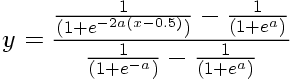
The Logistic Sigmoid

The so-called "Logistic Curve" is an elegant sigmoidal function which is believed by many scientists to best represent the growth of organic populations and many other natural phenomena. In software engineering, it is often used for weighting signal-response functions in neural networks. In this implementation, the parameter a regulates the slope or "growth rate" of the sigmoid during its rising portion. When a=0, this version of the Logistic function collapses to the Identity Function (y=x). The Logistic Sigmoid has very natural rates of change, but is expensive to calculate due to the use of many exponential functions.

//---------------------------------------
float logisticSigmoid (float x, float a){
  // n.b.: this Logistic Sigmoid has been normalized.

  float epsilon = 0.0001;
  float min_param_a = 0.0 + epsilon;
  float max_param_a = 1.0 - epsilon;
  a = max(min_param_a, min(max_param_a, a));
  a = (1/(1-a) - 1);

  float A = 1.0 / (1.0 + exp(0 -((x-0.5)*a*2.0)));
  float B = 1.0 / (1.0 + exp(a));
  float C = 1.0 / (1.0 + exp(0-a)); 
  float y = (A-B)/(C-B);
  return y;
}